In this blog post we study how a large amount of zeros in experiment data can affect causal inference. In an experiment, we ideally target users who qualify to receive a treatment, also known as triggered users. These are the users who can experience a meaningful effect (\(\Delta > 0)\). However, sometimes our targeting is not so precise. Or sometimes we realize later on that a segment of users is likely to experience \(\Delta = 0\). We use first principles to prove that including these “zero users” decreases both the average treatment effect as well as its standard error, but also decreases the t statistic of the two sample t test. However, under CUPED, it is possible to increase the t statistic. This is a peculiar phenomenon that we explain.

Previously we published a similar blog post on noncompliance, which is a form of zero users. This post is different in that it generalizes the types of users in the data to include a segment with a different mean, meant to illustrate a selection bias among the zero users and the triggered users.

Data Parameters

Say that we are in the typical AB test environment. There is a control group, with a metric \(y \sim N(\mu_C, \sigma^2_C)\). The treatment effect is a draw from \(\tau = N(\Delta, \sigma^2_\tau)\). The potential outcomes are related as \(y(1) = y(0) + \tau\) and thus \(E[y_T] = \mu_T = E[y_C] + \Delta\) and \(var(y_T) = \sigma^2_T = \sigma^2_C + \sigma^2_\tau\)

Now say there are some zeros in the data. Inside both the treatment group and the control group, there are users with \(y \sim N(\mu_z, \sigma^2_z)\). The mean and variance of this group can be distinct from the treatment and control parameters. This zero user group may be users that have not triggered yet, but nonetheless have a baseline. For these users, the treatment effect is exactly 0 without variability.

Imagine a dataset that has \(N\) total users, and for simplicity say \(N_T = N_C = 0.5N\). Within the treatment and control groups, say a user is a “zero-user” with probability \(p\). In the below sections we derive the average effect, its standard error, and the t statistic with the presence of zero users.

The Estimated ATE

The active part of the control group has mean \(\mu_C\). The zero part of the group has mean \(\mu_z\). The mean of the control group overall is \(E[y_{C, \text{observed}}] = (1-p)\mu_C + p\mu_z\). Likewise for the treatment group. The observed average treatment effect is \(\hat{\tau} = (1-p)\Delta\).

Variance of the ATE

The variance of this estimated treatment effect is \[\frac{2}{N} \cdot (Var(y_{T, \text{observed}}) + Var(y_{C, \text{observed}}))\]

The variance of the control group overall is derived from the Law of Total Variance. Say \(Z\) is a binary variable for whether the user is a zero user. Then \[Var(y) = E[Var(y|Z)] + Var(E[y | Z])\]. For \(Z = 1\), which happens with probability \(p\), the first term is \(E[Var(y|Z)] = \sigma^2_z\). For \(Z = 0\), it is \(\sigma^2_C\) with probability \((1-p)\).

To unpack the second term, \(E[y | Z] = \mu_z\) when \(Z = 1\), and is \(\mu_C\) when \(Z = 0\). The variance of these terms can be thought of as the variance of a scaled bernoulli random variable, so the variance of the control group is \[Var(E[y | Z]) = p (1-p) (\mu_z - \mu_C)^2\].

Finally, the variance of the estimated treatment effect is \[Var(\hat{\tau}) = \frac{2}{N} \biggl((1-p)(\sigma^2_T + \sigma^2_C) + 2p\sigma^2_z + p(1-p)((\mu_T - \mu_Z)^2 + (\mu_C - \mu_z)^2) \biggr)\]

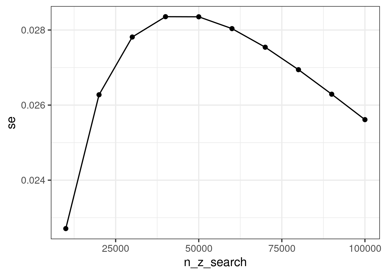
This formula has interesting properties. In general, we cannot guarantee that the variance of the effect is increasing or decreasing when zero-users are added.

Due to the \(\frac{1}{N}\) scaling factor, adding zero-users can decrease the variance of the effect.
If \(\mu_z\) is far away from \(\mu_T\), and \(\mu_C\), for example when there is a selection bias, then the variance can increase.
Note that under \(p = 0\), the variance of the effect is the normal variance of the active users.

Below is how we can implement the formulas in code.

zero_inflated_inference <- function(mu_C, mu_T, mu_z, sigma2_C, sigma2_T, sigma2_z, n_z, N) {
  p <- n_z / N
  
  mean_C_obs <- (1 - p) * mu_C + p * mu_z
  mean_T_obs <- (1 - p) * mu_T + p * mu_z
  ate_obs <- mean_T_obs - mean_C_obs
  
  var_C_obs <- (1 - p) * sigma2_C + p * sigma2_z + p * (1 - p) * (mu_C - mu_z)^2
  var_T_obs <- (1 - p) * sigma2_T + p * sigma2_z + p * (1 - p) * (mu_T - mu_z)^2
  se_obs <- sqrt((var_C_obs / (N/2)) + (var_T_obs / (N/2)))
  
  t_stat <- ate_obs / se_obs
  
  return (data.frame(
    ate = ate_obs,
    se = se_obs,
    t_statistic = t_stat,
    p_proportion = p,
    var_C_obs = var_C_obs,
    var_T_obs = var_T_obs
  ))
}

mu_C = 10
mu_T = 12
mu_z = 0
sigma2_C = 4
sigma2_T = 5
sigma2_z = 0.1
n_z = 200
n_a = 800
N = 1000
results <- zero_inflated_inference(
  mu_C, mu_T, mu_z,
  sigma2_C, sigma2_T, sigma2_z,
  n_z, N
)

print(results)

  ate        se t_statistic p_proportion var_C_obs var_T_obs
1 1.6 0.3042367    5.259062          0.2     19.22     27.06

With or without zeros?

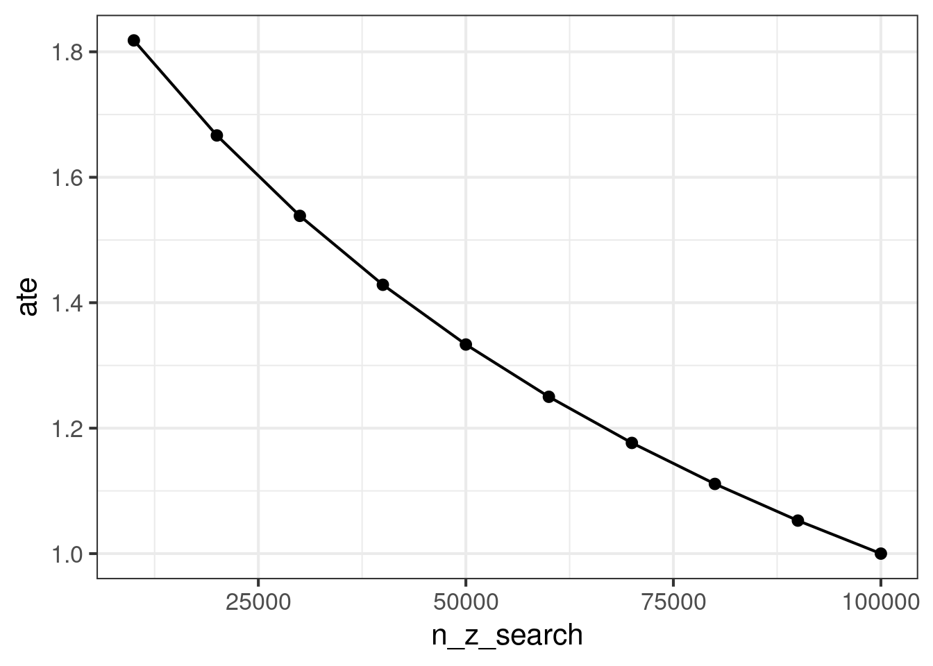
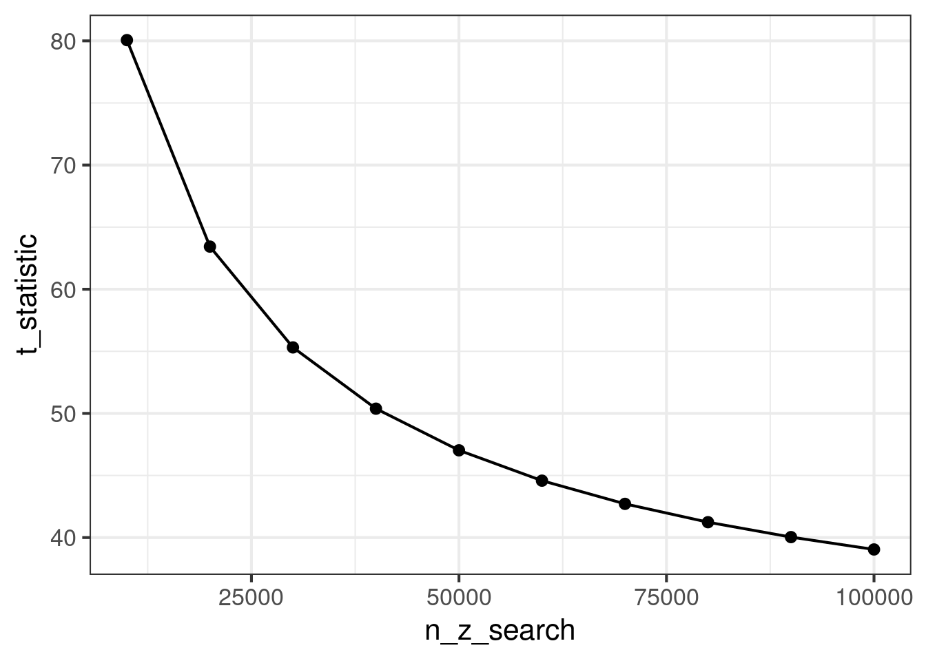
The estimated treatment effect is certainly diluted and decreases as we add more zero users. However, the variance is harder to understand. Nonetheless, the t statistic of the two sample t test is always decreasing. This is the intuition for why it is good to remove zero users as much as possible. Below, we demonstrate this phenomenon in simulation and then prove it from first principles.

n_z_search = seq(from = 10000, 100000, by = 10000)
results = map_dfr(n_z_search, function(n_z) {
  zero_inflated_inference(
    mu_C, mu_T, mu_z,
    sigma2_C, sigma2_T, sigma2_z,
    n_z, N = 100000 + n_z
  )
})

results %>%
  ggplot(aes(x = n_z_search, y = ate)) +
  geom_point() +
  geom_line() +
  theme_bw(base_size = 16)

results %>%
  ggplot(aes(x = n_z_search, y = se)) +
  geom_point() +
  geom_line() +
  theme_bw(base_size = 16)

results %>%
  ggplot(aes(x = n_z_search, y = t_statistic)) +
  geom_point() +
  geom_line() +
  theme_bw(base_size = 16)

Proof

Say there are two analyses, the “all” analysis and the “active” analysis. In order to see an increase in the t statistic, we must have

\[\frac{t_{all}}{t_{active}} = \sqrt{1-p} \sqrt{\frac{\sigma^2_C + \sigma^2_T}{\sigma^2_{C, \text{observed}} + \sigma^2_{T, \text{observed}}}} > 1\] To show that this is not possible, we will lower bound \(\sigma^2_{C, \text{observed}}\) and \(\sigma^2_{T, \text{observed}}\) For the control, we recall

\[\sigma^2_{C, \text{observed}} = (1-p)\sigma^2_C + p\sigma^2_z + p(1-p)(\mu_C - \mu_z)^2.\] Each individual term in this expression is nonnegative, so we can apply a bound \[\sigma^2_{C, \text{observed}} \geq (1-p)\sigma^2_C\] With a similar bound for the treatment. The sum is bounded \(\sigma^2_{C, \text{observed}} + \sigma^2_{T, \text{observed}} \geq (1-p)(\sigma^2_C + \sigma^2_T)\), therefore it is not possible for \(\frac{t_{all}}{t_{active}} > 1\).

A strange phenomenon under CUPED

Ironically, when the AB data is analyzed using CUPED, the t statistic can increase when zero users are added. The naive two sample t test uses the sample variance of the data to compute the t statistic. When the data is being modeled with covariates, the variance that we use is not the sample variance anymore, it is the residual variance after conditioning on covariates, \(X\). Say there is a covariate that is very predictive of whether a user is a zero user or not. Then all the variance that was introduced into the system by the zero user is explained away. The residual variance from the CUPED model will approach the variance of the active group. However, all the zero users will contribute to the total sample size, \(N\). This is what will decrease the variance of the estimated effect quickly, resulting in an increase t statistic. This is a very counter intuitive property.

We see this in code

zero_inflated_cuped_inference <- function(n_active = 10000, n_zero = 3000, effect_size = 0.5) {
  
  # Generate Active Users
  # y_post is a function of y_pre
  y_pre_active <- rnorm(n_active, mean = 10, sd = 2)
  y_post_active_control <- y_pre_active + rnorm(n_active, mean = 0, sd = 3)
  y_post_active_treat   <- y_pre_active + rnorm(n_active, mean = effect_size, sd = 3)
  
  # Generate Zero Users
  # y_post is almost just y_pre
  y_pre_zero  <- rnorm(n_zero, mean = 5, sd = 1)
  y_post_zero <- y_pre_zero + rnorm(n_zero, mean = 0, sd = 0.1) # Ultra-low residual variance
  
  # Combine into the "all" Dataframe
  df_all = rbind(
    data.frame(
      group = rep("Control", n_active),
      is_active = TRUE,
      pre = y_pre_active,
      post = y_post_active_control
    ),
    data.frame(
      group = rep("Control", n_zero),
      is_active = 0,
      pre = y_pre_zero,
      post = y_post_zero
    ),
    data.frame(
      group = rep("Treatment", n_active),
      is_active = TRUE,
      pre = y_pre_active,
      post = y_post_active_treat
    ),
    data.frame(
      group = rep("Treatment", n_zero),
      is_active = 0,
      pre = y_pre_zero,
      post = y_post_zero
    )
  )
  
  df_triggered <- df_all %>% filter(is_active == TRUE)
  t_triggered <- t.test(post ~ group, data = df_triggered)$statistic
  
  t_total_std <- t.test(post ~ group, data = df_all)$statistic
  
  model_cuped <- lm_robust(post ~ group + pre, data = df_all)
  t_total_cuped <- summary(model_cuped)$coefficients["groupTreatment", "t value"]
  
  return(data.frame(
    Analysis = c("Active", "All", "All (CUPED)"),
    T_Statistic = c(t_triggered, t_total_std, t_total_cuped)
  ))
}

set.seed(100)
results <- zero_inflated_cuped_inference()
print(results)

     Analysis T_Statistic
1      Active  -10.339967
2         All   -8.408577
3 All (CUPED)   12.359841

Things to revise for next version

Why was there a sign change above?

In order for the all analysis to be better, we need the correlation between pre and post to have

\[\rho^2_{\text{all}} > 1 - (1-p)(1 - \rho^2_{\text{active}})\]