Statistical power is a concept that helps us plan for an effective experiment. Power is typically described in terms of a purely randomized and controlled trial, where we can take advantage of certain properties like independence. It is also typically described in the context of measuring the difference in means, which also has properties like the Central Limit Theorem that it takes advantage of. Finally, an assumption in typical description is that all units that are assigned to the treatment group are successfully treated, and all units assigned to the control are successfully withheld.
But not all experiments are so perfectly planned and executed. It is important to understand the history of how statistical power was derived, from first principles, so that we can adapt it and innovate. For example, some experiments do not have perfect compliance. Many experiments will try to give treatment to a subject, but that subject refuses, or forgets, to use the treatment. This complexity can add layers to the question: “what should we measure? The average effect or the average effect among the compliers?” With this complication we will need to revisit our formula for statistical power. We will do this innovation exercise in the next post. For now, let us understand the history of statistical power.
Power is always associated with a hypothesis test. \[\text{Power} = 1 - \beta = P(\text{Reject }H_0 | H_A)\] where \(\alpha\) is the type 1 error rate, and \(\beta\) is the type 2 error rate.
So to derive power, we must first identify the rejection rules of the hypothesis test, then evaluate the probability of rejection if the alternative is true.
To illustrate, we specify a very generic hypothesis test, the difference in means. While frequently associated with the t test, it is not necessarily tied to it. The hypothesis about the difference in means is
From the Central Limit Theorem, we know the distribution of a sample mean is \(\bar{X} \sim N(\mu, \sigma^2 / n)\) and the standard error on \(\bar{X}\) is \(se(\bar{X}) = \sigma/\sqrt{n}\). The Z statistic is a transformation with \(Z = \frac{\bar X - \mu}{se(\bar{X})} \sim N(0, 1)\). Now we apply information from the hypothesis test, where the mean in question is the difference in two means.
Rejection Rule
In order to reject the null, we must first assume that the null is true. Then we must show that the sample mean for \(\Delta\) is sufficiently different from 0, even when the true governing parameter is 0. This is conveniently done by working with the normalized Z statistic. In the case of the null, the sample mean \(\bar{\Delta} \sim N(\Delta, \sigma^2)\) and \(\Delta = 0\). Converting to a normalized Z statistic we have \(Z = \frac{\bar{\Delta}}{{SE(\bar{\Delta})}} \sim N(0, 1)\). Now, we can state the rejection rule: reject if \(|Z| \geq z_{1-\alpha/2}\). Equivalently \[\begin{align}
\left|\frac{\bar{\mu}_1 - \bar{\mu}_0}{se(\bar{\Delta})}\right| &\geq z_{1-\alpha/2}
\end{align}\] where \(se(\bar{\Delta}) = \sqrt{\frac{\sigma^2}{n_T} + \frac{\sigma^2}{n_C}}\) under randomization. If \(n_T = k \cdot n_C\), then we can use the reduction
Power is the probability of triggering the rejection rules, which were derived under the null \(H_0: \Delta = 0\), when the true data generating process has \(\Delta \neq 0\). It is important to understand which governing parameter is in play here. The rejection rules will be derived using \(\Delta = 0\), and those rules will be fixed. Then, we toggle the governing parameter to have \(\Delta \neq 0\), and benchmark the probability that data under this governing parameter will hit the rejection rule.
Say that \(H_A\) is true and there are two distinct means \(\mu_0\) and \(\mu_1\) with \(\mu_1 - \mu_0 = k \neq 0\). Under \(H_A\) we cannot claim the usual Z statistic is distributed N(0, 1). Instead, we have
\[\begin{align}
Z | H_A &= \frac{\bar{\Delta}}{se(\bar{\Delta})} \sim N(\frac{k}{se(\bar{\Delta})},1) \\
\end{align}\]
Now we revisit the rejection rule: reject when \(|Z| \geq z_{1-\alpha/2}\). Power is the probability of triggering the rejection rule when \(H_A\) is true, so
\[\begin{align}
Power &= P(|Z| \geq z_{1-\alpha/2} | Z \sim N(\frac{k}{se(\bar{\Delta})}, 1))
\end{align}\]
Let \(\delta = \frac{\Delta | H_A}{se(\bar{\Delta})}\) be the noncentrality parameter (ncp), using the anticipated effect size we would like to detect under \(H_A\). The ncp is a parameter we will revisit many times. The final solution for power is \[
\boxed{\text{Power} = \Phi(\delta - z_{1-\alpha/2}) + \Phi(-\delta - z_{1-\alpha/2})}
\]
power.t.test(n = n * treatment_share,delta = treatment_effect,sd =sqrt(sigma2),strict =TRUE)
     Two-sample t test power calculation

              n = 500
          delta = 0.01
             sd = 1.414214
      sig.level = 0.05
          power = 0.05143037
    alternative = two.sided

NOTE: n is number in *each* group
How Power Changes
A lot of research in experimentation goes into methods to increase statistical power. Using the formula, the variables that drive power are:
The treatment effect, \(\mu_1 - \mu_0\).
The critical value, determined by \(\alpha\).
Sample size, \(n\).
Variance, \(\sigma^2\).
By changing the treatment effect that we want to detect, we can change power. However, that may jeopardize the practical value of an experiment. If we only power our experiment to detect large treatment effects that in practice do not happen, then the experiment is useless. Increasing \(\alpha\) is also a simple change, but it also increases the false positive rate. Increasing sample size decreases the standard error, but it will take more time and resources to accumulate the extra data.
Finally, the last path to improve power has a lot of subtlety. The role variance plays in the power formula is not fixed, it can vary. Its role is more precisely called “unexplained variance”. If there is a model that relates the metric, \(y\), with the treatment variable and exogeneous covariates, \(X\), then \(\sigma^2\) is actually \(\text{Var}(y | X)\), or equivalently the variance of the residuals after we use \(X\) to explain part of the variance. Using a good set of \(X\) variables, we can make the unexplained variance small.
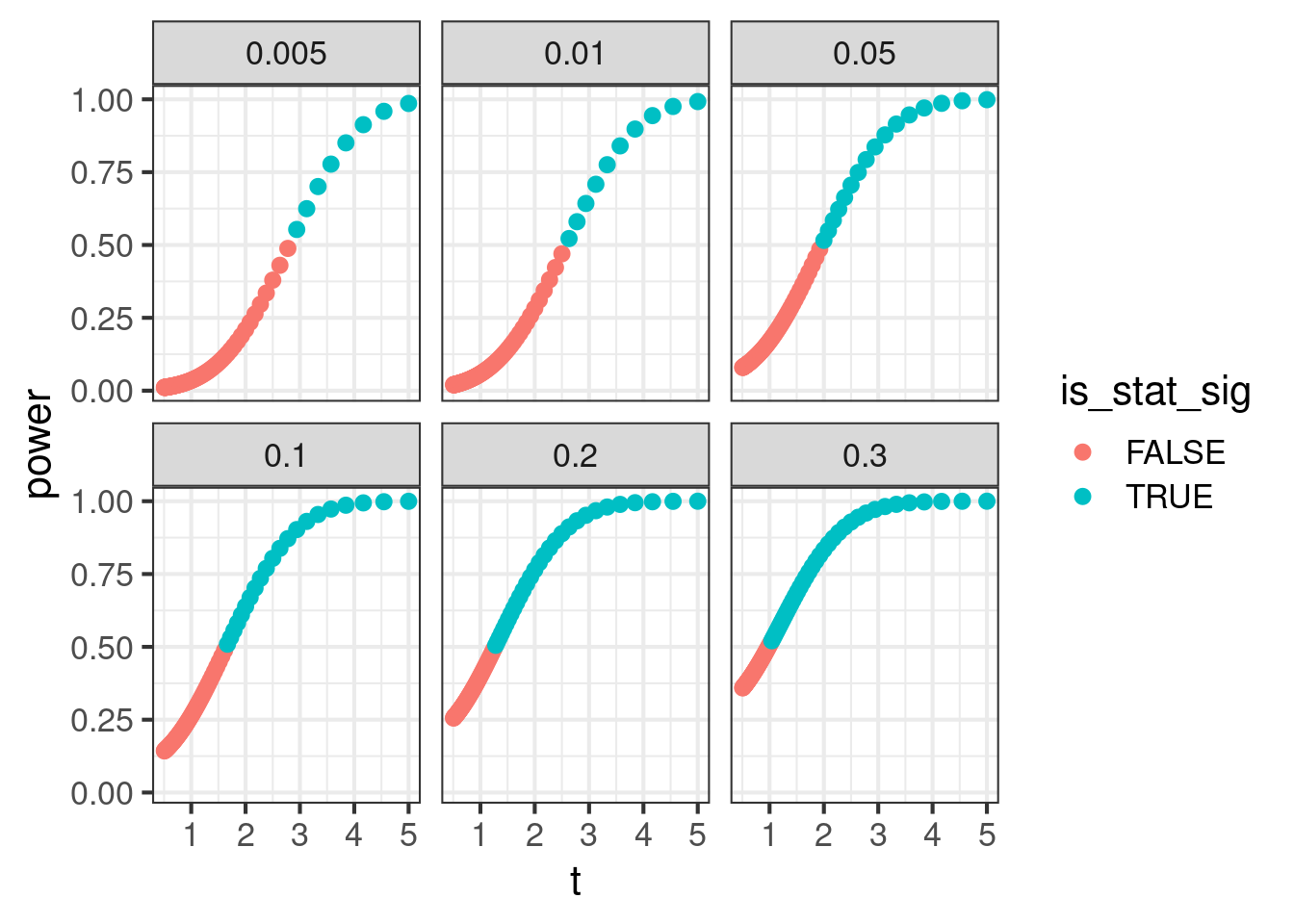
Which of these levers should we pursue to get maximal power? How much will power change? To answer this, we combine \(n\) and variance into the more general variable, standard error. We merge the standard error and the effect size using the more general variable \(\delta\). Below we plot power as \(\delta\) and \(\alpha\) vary. If we wanted to unpack the specific sensitivity to standard error, we could say the sensitivity of power to standard error is
It is a function of ncp and \(\alpha\), and the sensitivity is charted below.
power =function(delta, se, alpha = .05) { pooled_ncp = delta / se crit =qnorm(1-alpha/2)pnorm(-crit - pooled_ncp) + (pnorm(-crit + pooled_ncp))}
MDE as the Inverse of Statistical Power
MDE is the minimum detectable effect. It operates as the inverse to statistical power. Instead of asking: how much power do I have given an effect size and standard error, it asks: what is the effect size I can detect given a fixed amount of power and standard error.
To derive the MDE from first principles, we go back to the definition of power and how it is framed in terms of the rejection rule:
This equation about the CDF can be simplified. The noncentrality parameter is distributed \(\delta \sim N(0, 1)\), so it being greater than or equal to \(z_{1-\alpha/2}\) is actually just \(1 - \Phi(z_{1-\alpha/2} - \delta)\). Then the derivation for the MDE is
Using common numbers, \(\alpha = 0.05\), \(\beta = 0.2\), the rule of thumb for MDE is
\[
MDE = 2.8 \cdot SE
\] or equivalently we need a ncp of \(2.8\).
Let’s unpack this common rule of thumb explicitly. It says that the smallest effect size we can detect while ensuring an 80% power is \(2.8 \cdot se(\bar{\Delta})\). (The SE here is the residual standard error after controlling for other variables.)
This looks like a similar rule of thumb related to rejecting the null: reject if the effect size is larger than 1.96 SE. This separate rule of thumb can be very confusing - why are there two different constants of 1.96 and 2.8? This rule describes when can we flag a result as stat sig while ensuring a different property: that under the null hypothesis there is less than a 5% chance of generating this effect by random. This rule of thumb is offering a different guarantee, not one about power. Ensuring 80% power at a specific effect size simply says that there is a good chance we can detect these effects, but it does not make it impossible. Even using power = 50% we will correctly flag some results as stat sig. (See multiple online discussions like this one) 1.96 SE is a rejection rule after the test executes, while 2.8 SE is a rule for planning to ensure 80% power. However, it is noteworthy that the scientific community is advocating for rejecting at 2.8 SE, or equivalently a p value of 0.005. (See Redefine Statistical Significance)
Sample Size Calculator
It’s easier for a business to think about designing an experiment around the MDE. It’s a more natural discussion: what is the smallest effect that the business would still care about?
Given an MDE, we pivot the problem again. If \(se(\bar{\Delta}) = \sqrt{\frac{\sigma_T^2}{n_T} + \frac{\sigma_C^2}{n_C}} = \sqrt{Var(\bar{y}_c) (1 + \frac{1}{k})}\), and \(n_T = k \cdot n_C\), then