Bayesian Universal Modeling

In the conditionally sufficient statistics post, a streaming service prompted households to turn on a new playback setting and measured how it changed hours watched and rebuffers per play. One universal model handled everything that made that experiment hard: households with several profiles, a prompt that profiles could ignore, a ramp from 5% to 50% of new accounts, and a ratio metric. It reported each effect with a standard error, and it could do so from a compressed dataset of 8 rows.

The product manager reads the report and asks a different question: what is the probability that the setting cuts rebuffers per play by at least 10% for the profiles that use it? A standard error does not answer that. A posterior distribution does, and in the posterior distribution post we argued that a posterior is what decision makers want. The bootstrap post showed how to get one for a least squares fit without writing a likelihood, with the Bayesian bootstrap.

This post combines the two. We first show that the Bayesian bootstrap gives a posterior for every design the universal model covers, and then that it can be computed in one pass over the data, or from the compressed dataset itself.

The data in this post is synthetic and the scenario is educational. It does not describe a production system.

The Universal Model

The experiment

We use the same simulated experiment as the previous post. Each account \(a\) enters on \(\text{day}_a \in \{1, 2, 3, 4\}\) and is prompted, \(Z_a = 1\), with probability \(e_{\text{day}}\), which ramps from 5% to 50%. Each profile \(p\) of the account has covariates measured before the experiment: hours per day \(x_1\), tenure \(x_2\), whether it is a kids profile, and its main device, coded as the indicators mobile and web. A prompted profile turns the setting on, \(T_{ap} = 1\), if it is a complier. We measure its hours per day \(y_{ap}\), its plays \(D_{ap}\) and its rebuffers \(N_{ap}\).

The code is the code of the previous post, folded. It simulates the 20,000 accounts, prepares the profile rows, and fits the universal model with its cluster robust standard errors. The only change is that the coefficient matrix is called beta, because in this post \(B\) is the number of posterior draws.

simulate_accounts <- function(n_accounts = 20000, propensity = c(0.05, 0.10, 0.25, 0.50), force_Z = NULL,
                              full_compliance = FALSE, one_profile = FALSE) {
  accounts <- tibble(
    account = seq_len(n_accounts),
    day = sample.int(length(propensity), n_accounts, replace = TRUE, prob = rev(seq_along(propensity))),
    n_profiles = if (one_profile) 1L else pmin(1L + rpois(n_accounts, 1.2), 5L),
    quality = rnorm(n_accounts, 0, 0.5),                       # shared by the account's profiles
    engagement = rnorm(n_accounts, 0, 0.5)                     # account part of engagement
  ) |>
    mutate(Z = rbinom(n(), 1, propensity[day]), Z = if (is.null(force_Z)) Z else force_Z)
  accounts[rep(accounts$account, accounts$n_profiles), ] |>
    mutate(
      profile = sequence(accounts$n_profiles),
      kids = rbinom(n(), 1, if_else(profile == 1, 0.05, 0.3)),
      device = sample(c("tv", "mobile", "web"), n(), replace = TRUE, prob = c(0.5, 0.35, 0.15)),
      engagement_p = engagement + rnorm(n(), 0, 0.8),          # the profile's engagement, not observed
      x1 = rlnorm(n(), 0.7 - 0.12 * day - 0.6 * kids + 0.3 * engagement_p, 0.6),
      x2 = rgamma(n(), 2, 1) * (1.2 - 0.15 * day),
      complier = rbinom(n(), 1, plogis(-0.3 + 0.5 * log(x1) + 0.6 * engagement_p - 0.8 * kids)),
      T = if (full_compliance) Z else Z * complier,
      y = 0.5 + 0.8 * x1 + 0.1 * x2 + 0.5 * engagement_p + quality +
        T * (0.3 + 0.15 * x1 - 0.2 * kids) + rnorm(n(), 0, 0.5 + 0.3 * x1),
      D = 1 + rpois(n(), exp(1 + 0.4 * log(x1) + 0.3 * engagement_p + 0.2 * (device == "tv")) * (1 + 0.15 * T)),
      N = rpois(n(), D * 0.08 * exp(-0.4 * T * (1 + 0.5 * (device == "mobile")) + 0.4 * quality - 0.2 * engagement_p))
    )
}

propensity <- c(0.05, 0.10, 0.25, 0.50)
x_cols <- c("x1", "x2", "kids", "mobile", "web")
x_ref <- c(x1 = 2, x2 = 2, kids = 0, mobile = 0, web = 0)
y_cols <- c("y", "N", "D", "TN", "TD")
d <- length(x_cols) + 1                              # intercept and k covariates
o <- length(y_cols)                                  # number of outcome columns

prepare <- function(profiles, ramp = TRUE) {
  e_hat <- profiles |>
    distinct(account, day, Z) |>
    group_by(day) |>
    summarise(e_hat = mean(Z))
  profiles |>
    left_join(e_hat, by = "day") |>
    mutate(w = if (ramp) if_else(Z == 1, 1 / e_hat, 1 / (1 - e_hat)) else 1,     # inverse propensity weight
           mobile = as.numeric(device == "mobile"), web = as.numeric(device == "web"),
           TN = T * N, TD = T * D)
}

centered <- function(df) {
  r <- cbind(1, sweep(as.matrix(df[x_cols]), 2, x_ref))
  colnames(r) <- c("1", paste0(x_cols, "_c"))
  r
}

design <- function(df) {
  r <- centered(df)
  list(M_1 = cbind(r, `colnames<-`(df$Z * r, paste0("Z*", colnames(r)))),     # first stage: instruments
       M_2 = cbind(r, `colnames<-`(df$T * r, paste0("T*", colnames(r)))))     # second stage: regressors
}

fit_rows <- function(df) {
  m <- design(df)
  Y <- as.matrix(df[y_cols])
  M1_W_M2 <- crossprod(m$M_1 * df$w, m$M_2)
  beta <- solve(M1_W_M2, crossprod(m$M_1 * df$w, Y))
  eps <- Y - m$M_2 %*% beta
  inner <- do.call(cbind, map(seq_len(o), \(l) rowsum(m$M_1 * (df$w * eps[, l]), df$account)))
  M1_W_M2_inv <- kronecker(diag(o), solve(M1_W_M2))
  list(beta = beta, V = M1_W_M2_inv %*% crossprod(inner) %*% t(M1_W_M2_inv))
}

complier_mean <- function(df) {
  if (all(df$T == df$Z)) return(colSums(df$w * df[x_cols]) / sum(df$w))
  arm <- df |>
    group_by(Z) |>
    summarise(across(all_of(x_cols), \(v) sum(w * T * v) / sum(w)), T = sum(w * T) / sum(w))
  unlist(arm[arm$Z == 1, x_cols] - arm[arm$Z == 0, x_cols]) / (arm$T[arm$Z == 1] - arm$T[arm$Z == 0])
}

gradient <- function(f, theta, kappa = 1e-20) {
  map_dbl(seq_along(theta), \(i) Im(f(theta + 1i * kappa * (seq_along(theta) == i))) / kappa)
}

effect_functions <- function(x_C, x_ref, cols) {
  delta <- c(rep(0, length(x_ref) + 1), 1, x_C - x_ref)
  line <- \(beta, col) sum(delta * beta[, col])
  effect_list <- list(tau_LATE = \(beta) line(beta, "y"))
  if ("TN" %in% cols) effect_list$tau_R <- \(beta) line(beta, "TN") / line(beta, "TD") -
    (line(beta, "TN") - line(beta, "N")) / (line(beta, "TD") - line(beta, "D"))
  effect_list
}

effects <- function(fit, x_C, x_ref) {
  effect_list <- effect_functions(x_C, x_ref, colnames(fit$beta))
  theta <- as.vector(fit$beta)
  map_dfr(names(effect_list), \(nm) {
    f <- \(th) effect_list[[nm]](matrix(th, nrow(fit$beta), dimnames = list(NULL, colnames(fit$beta))))
    grad <- gradient(f, theta)
    tibble(effect = nm, estimate = Re(f(theta)), se = sqrt(drop(t(grad) %*% fit$V %*% grad)))
  })
}

set.seed(2026)
profiles <- simulate_accounts()
df <- prepare(profiles)
fit <- fit_rows(df)
x_C <- complier_mean(df)
css <- effects(fit, x_C, x_ref)
css

# A tibble: 2 × 3
  effect   estimate      se
  <chr>       <dbl>   <dbl>
1 tau_LATE   0.664  0.0572 
2 tau_R     -0.0255 0.00410

The model

The universal model is two stage least squares with weights and cluster robust standard errors. With the covariates centered at a fixed reference point, \(x_{ap}\) standing for \(x_{ap} - x_{ref}\), its two stages are

\[\begin{align} y_{ap} &= \underbrace{\beta_{00} + x_{ap}^\top \beta_{0x}}_{\text{baseline line}} + T_{ap} \underbrace{\left(\beta_{10} + x_{ap}^\top \beta_{1x}\right)}_{\text{treatment line}} + \varepsilon_{ap} && \text{second stage} \\ T_{ap} &= \gamma_{00} + x_{ap}^\top \gamma_{0x} + Z_a \left(\gamma_{10} + x_{ap}^\top \gamma_{1x}\right) + \nu_{ap} && \text{first stage for } T \\ T_{ap} x_{apj} &= \gamma^{(j)}_{00} + x_{ap}^\top \gamma^{(j)}_{0x} + Z_a \left(\gamma^{(j)}_{10} + x_{ap}^\top \gamma^{(j)}_{1x}\right) + \nu^{(j)}_{ap} && \text{first stage for interaction } j = 1, \dots, k \end{align}\]

with \(k = 5\) covariates. Each account carries the inverse propensity weight \(w_a = 1/\hat e_{\text{day}}\) if prompted and \(w_a = 1/(1 - \hat e_{\text{day}})\) if not, where \(\hat e_{\text{day}}\) is the share of that day’s accounts that were prompted. One fit holds five outcome columns: hours \(y\), rebuffers \(N\), plays \(D\), and \(TN\) and \(TD\), which equal \(N\) and \(D\) for profiles with the setting on and 0 otherwise.

Stacking the instruments \(m_{1,ap} = (1, x_{ap}, Z_a, Z_a x_{ap})\) into \(M_1\), the regressors \(m_{2,ap} = (1, x_{ap}, T_{ap}, T_{ap} x_{ap})\) into \(M_2\), and the weights into \(W = \text{diag}(w)\), the coefficients are

\[\hat\beta = (M_1^\top W M_2)^{-1} M_1^\top W Y,\]

a \(2(k+1) \times 5\) matrix with one column per outcome, \(\hat\beta_y, \hat\beta_N, \hat\beta_D, \hat\beta_{TN}, \hat\beta_{TD}\).

The model rests on three assumptions about the design.

(A1) Accounts are independent of each other. Profiles of the same account may be correlated in any way.

(A2) Within a cohort, the prompt is randomized with probability \(e_{\text{day}}\), independently of everything else.

(A3) The prompt affects a profile’s outcomes only through \(T\), and no profile turns the setting on only when it is not prompted.

The effects

The treatment line is fit to the compliers, so the effect for the compliers, the LATE, is the treatment line read at the compliers’ mean covariates \(\bar x_C\), estimated as a ratio of two intent to treat effects:

\[\begin{align} \tau_{LATE} &= \beta_{10} + (\bar x_C - x_{ref})^\top \beta_{1x}, \\ \bar x_C &= \frac{E[T x \mid Z = 1] - E[T x \mid Z = 0]}{E[T \mid Z = 1] - E[T \mid Z = 0]}. \end{align}\]

Write \(\ell_N\) for the treatment line of the outcome \(N\) read at \(\bar x_C\), and similarly for the other outcomes. Then \(\ell_{TN}\) is the compliers’ mean rebuffers with the setting on, \(E[N(1) \mid C]\), and \(\ell_{TN} - \ell_N\) is their mean rebuffers with it off, \(E[N(0) \mid C]\). The effect on rebuffers per play is

\[\tau_R = \frac{\ell_{TN}}{\ell_{TD}} - \frac{\ell_{TN} - \ell_N}{\ell_{TD} - \ell_D}.\]

The product manager’s question is about the relative change in rebuffers per play,

\[\rho_R = \frac{\ell_{TN} / \ell_{TD}}{(\ell_{TN} - \ell_N) / (\ell_{TD} - \ell_D)} - 1,\]

a third function of the same coefficients. The previous post computed standard errors with the delta method, which needs the gradient of each effect and the joint covariance of all the coefficients. Because we simulated the data, we know the true effects. We simulate the same accounts twice, once with every account prompted and once with none, and compare the compliers in the two worlds.

truth_pair <- function(seed, n_accounts = 1e6) {
  set.seed(seed)
  p1 <- simulate_accounts(n_accounts, force_Z = 1)
  set.seed(seed)
  p0 <- simulate_accounts(n_accounts, force_Z = 0)
  C <- p1$complier == 1                                      # the same profiles comply in both worlds
  rate_1 <- sum(p1$N[C]) / sum(p1$D[C])
  rate_0 <- sum(p0$N[C]) / sum(p0$D[C])
  c(tau_LATE = mean(p1$y[C] - p0$y[C]), tau_R = rate_1 - rate_0, rho_R = rate_1 / rate_0 - 1)
}
truth <- colMeans(do.call(rbind, map(1:2, truth_pair)))
invisible(gc())
truth

   tau_LATE       tau_R       rho_R 
 0.61334648 -0.02724864 -0.37012026 

The compressed dataset

The previous post compressed the profile rows in two steps. Each account becomes an account summary \(u_a\), the vector of the sums over its profiles

\[S^Y_a = \sum_p \begin{pmatrix} 1 \\ x_{ap} \end{pmatrix} y_{ap}^\top, \qquad S_a = \sum_p \begin{pmatrix} 1 \\ x_{ap} \end{pmatrix} \begin{pmatrix} 1 & x_{ap}^\top \end{pmatrix}, \qquad S^T_a = \sum_p T_{ap} \begin{pmatrix} 1 \\ x_{ap} \end{pmatrix} \begin{pmatrix} 1 & x_{ap}^\top \end{pmatrix},\]

where \(y_{ap}\) is the row of all outcome columns. Accounts with the same prompt and cohort share \(Z_a\) and \(w_a\), so each stratum \(h = (Z, \text{day})\) becomes one compressed row with three fields: the number of accounts \(G_h\), the first moments \(\sum_{a \in h} u_a\), which give \(\hat\beta\), and the second moments \(\sum_{a \in h} u_a u_a^\top\), which give the cluster robust covariance. The compressed dataset has 8 compressed rows.

Why a Posterior

The previous post’s report reads: the LATE on hours is 0.664 with a standard error of 0.057, and the effect on rebuffers per play is -0.0255 with a standard error of 0.0041. These describe a sampling distribution. The standard error says how much the estimate would move if we reran the experiment on new accounts, while the effect stays fixed. As the posterior distribution post explained, that does not support the statement “there is a 95% probability that the effect is in this interval”, and it does not answer the product manager. A posterior, \(p(\tau \mid \text{data})\), does both: it treats the effect as uncertain and the data as fixed, so the probability that \(\rho_R < -10\%\) is the share of the posterior below \(-10\%\).

A conjugate Bayesian model for this experiment would be hard to write. It would need a likelihood for hours, rebuffers and plays jointly, correlated within accounts, with a first stage for compliance, and it would be wrong in ways that make the posterior too narrow, as we saw for the Gaussian likelihood in the bootstrap post. That post showed the alternative. The Bayesian bootstrap puts the prior and the likelihood on the population instead of on the model, and the model is used only to define which summary of the population we want. The universal model is a summary of the population like any other, so the same idea should work. The rest of this post checks whether it does, and how to compute it at scale.

A Posterior for the Universal Model

The unit that gets a weight is the account

The Bayesian bootstrap treats the population as a mix of the units we observed, in unknown shares, and draws the shares from their posterior. The unit has to be the unit of independence. Here that is the account, by (A1): profiles of the same account are correlated, so a population is a mix of whole accounts, each with all its profiles. We add the two assumptions of the bootstrap post at the level of accounts.

(A4) The population contains only the kinds of accounts we observed. Writing \(F_a\) for the population made only of copies of account \(a\), with its cohort, prompt, profiles and outcomes, the population is \(F = \sum_a \pi_a F_a\) for unknown shares \(\pi_a \geq 0\) that add up to 1.

(A5) The prior on the shares \(\pi = (\pi_1, \dots, \pi_G)\), where \(G\) is the number of accounts, is a Dirichlet distribution with zero pseudo-counts.

As the bootstrap post derived, the posterior of \(\pi\) is then Dirichlet\((1, \dots, 1)\), and a draw is

\[\pi_a = \frac{\xi_a}{\sum_{a'} \xi_{a'}}, \qquad \xi_a \overset{\text{iid}}{\sim} \text{Exponential}(1).\]

\(\xi_a\) is the account’s bootstrap weight. It is a weight but not a probability weight; \(\pi_a\) is the probability weight. Every profile of an account shares the account’s bootstrap weight.

The effects as functions of the population

To compute an effect on a drawn population, we write each step of the universal model as a function of \(F\). With \(F = \sum_a \pi_a F_a\), an average over \(F\) is a \(\pi\)-weighted average over our accounts.

1. The propensity. The share of a cohort’s accounts that were prompted is \[e_{\text{day}}(F) = \frac{\sum_{a \in \text{day}} \pi_a Z_a}{\sum_{a \in \text{day}} \pi_a},\] and the inverse propensity weights \(w_a(F)\) follow from it. Each draw of the population has its own share of prompted accounts, so the propensity is recomputed in every draw.
2. The coefficients. The universal model solves \(\sum_a w_a \sum_p m_{1,ap} (y_{ap} - m_{2,ap}^\top \beta) = 0\) on our sample. On the population \(F\) the sum over accounts becomes a \(\pi\)-weighted sum, so the solution is \[\beta(F) = \Big(\sum_a \pi_a w_a(F) \sum_p m_{1,ap} m_{2,ap}^\top\Big)^{-1} \sum_a \pi_a w_a(F) \sum_p m_{1,ap} y_{ap}^\top,\] which is the universal model fit with the combined weight \(\pi_a w_a(F)\) on every profile of account \(a\).
3. The compliers’ mean. \(\bar x_C(F)\) is the ratio of intent to treat effects, with each expectation a weighted average with weights \(\pi_a w_a(F)\).
4. The effects. \(\tau_{LATE}(F)\), \(\tau_R(F)\) and \(\rho_R(F)\) are the same functions of \(\beta(F)\) and \(\bar x_C(F)\) as before.

Every step is unchanged when all the \(\pi_a\) are multiplied by the same constant: the propensity is a ratio, and the constant cancels between the inverse and the second sum of \(\beta(F)\), and in the ratio \(\bar x_C(F)\). So we can use the bootstrap weights \(\xi_a\) directly, without normalizing them. With all \(\xi_a = 1\) the steps reproduce the estimates of the previous post exactly.

At the true population, \(\tau_{LATE}(F)\) is the LATE: the previous post derived that the treatment line is fit to the compliers’ effects under (A1)–(A3), and that derivation holds for any population that satisfies them. The posterior of \(\tau_{LATE}(F)\) is therefore a posterior for the LATE.

One draw, step by step

draw_rows computes the three effects on the profile rows for one vector of bootstrap weights, one per account. It recomputes the propensity, refits the model with the combined weights, and recomputes the compliers’ mean. rows_data prepares the matrices once, because they do not change across draws.

rows_data <- function(df) {
  accounts <- df |>
    distinct(account, day, Z) |>
    arrange(account)
  stopifnot(all(accounts$account == seq_len(nrow(accounts))))   # accounts numbered 1, 2, ...
  c(design(df), list(Y = as.matrix(df[y_cols]), r = centered(df), account = df$account, Z = df$Z, T = df$T,
                     accounts = accounts))
}

effect_values <- function(beta, x_C_c) {        # x_C_c: the compliers' mean in centered units
  delta <- c(rep(0, d), 1, x_C_c)
  l <- colSums(delta * beta)                     # each outcome's treatment line at the compliers' mean
  rate_1 <- l[["TN"]] / l[["TD"]]
  rate_0 <- (l[["TN"]] - l[["N"]]) / (l[["TD"]] - l[["D"]])
  c(tau_LATE = l[["y"]], tau_R = rate_1 - rate_0, rho_R = rate_1 / rate_0 - 1)
}

draw_rows <- function(rows, xi, ramp = TRUE, encouraged = TRUE) {
  acc <- rows$accounts
  # 1. The propensity: the xi-weighted share of each cohort's accounts that were prompted
  e_day <- rowsum(xi * acc$Z, acc$day)[, 1] / rowsum(xi, acc$day)[, 1]
  w <- if (ramp) if_else(acc$Z == 1, 1 / e_day[acc$day], 1 / (1 - e_day[acc$day])) else 1
  # 2. The coefficients, with the combined weight xi_a w_a on every profile of account a
  w_ap <- (xi * w)[rows$account]
  beta <- solve(crossprod(rows$M_1 * w_ap, rows$M_2), crossprod(rows$M_1 * w_ap, rows$Y))
  colnames(beta) <- y_cols
  # 3. The compliers' mean: ratio of the weighted intent to treat effects on T (1, x) and T
  x_C_c <- if (encouraged) {
    arm <- \(z) colSums(rows$r * (w_ap * rows$T * (rows$Z == z))) / sum(w_ap * (rows$Z == z))
    diff <- arm(1) - arm(0)
    diff[-1] / diff[1]
  } else colSums(rows$r * w_ap)[-1] / sum(w_ap)
  # 4. The effects
  effect_values(beta, x_C_c)
}

rows <- rows_data(df)
draw_rows(rows, rep(1, nrow(rows$accounts)))

   tau_LATE       tau_R       rho_R 
 0.66391019 -0.02547824 -0.33778566 

With every bootstrap weight equal to 1, the draw reproduces the estimates of the previous post, 0.6639 for the LATE and -0.02548 for the ratio. Now we draw one vector of bootstrap weights. Here are the profile rows of two accounts, a prompted one and an unprompted one, with their weights:

set.seed(1)
xi <- rexp(nrow(rows$accounts))
example_accounts <- c(
  df |>
    group_by(account) |>
    filter(first(Z) == 1, n() >= 3, any(T == 1), any(T == 0)) |>
    pull(account) |>
    first(),
  df |>
    group_by(account) |>
    filter(first(Z) == 0, n() >= 2) |>
    pull(account) |>
    first())
df |>
  filter(account %in% example_accounts) |>
  mutate(xi = xi[account]) |>
  select(account, profile, day, Z, T, x1, y, w, xi)

# A tibble: 7 × 9
  account profile   day     Z     T    x1      y     w    xi
    <int>   <int> <int> <int> <int> <dbl>  <dbl> <dbl> <dbl>
1       1       1     2     0     0 1.89  0.0541  1.12 0.755
2       1       2     2     0     0 0.867 0.377   1.12 0.755
3      15       1     1     1     1 1.67  3.02   19.5  1.05 
4      15       2     1     1     0 2.21  1.96   19.5  1.05 
5      15       3     1     1     0 0.704 0.426  19.5  1.05 
6      15       4     1     1     0 0.481 0.173  19.5  1.05 
7      15       5     1     1     0 5.61  4.87   19.5  1.05 

Each account’s weight is shared by its profiles. In this draw the prompted account 15 counts 1.05 times, and the unprompted account 1 counts 0.76 times. The drawn population also has its own propensities:

rows$accounts |>
  mutate(xi = xi) |>
  group_by(day) |>
  summarise(e_hat = mean(Z), e_draw = sum(xi * Z) / sum(xi))

# A tibble: 4 × 3
    day  e_hat e_draw
  <int>  <dbl>  <dbl>
1     1 0.0512 0.0530
2     2 0.106  0.104 
3     3 0.247  0.248 
4     4 0.499  0.497 

e_hat is the share prompted in our sample, and e_draw is the share in the drawn population. They differ by a fraction of a percentage point, and the inverse propensity weights follow e_draw. The draw’s effects are

draw_rows(rows, xi)

   tau_LATE       tau_R       rho_R 
 0.63926109 -0.03505879 -0.43253513 

The posterior

We repeat this with \(B = 1{,}000\) draws.

set.seed(2)
B <- 1000
Xi <- matrix(rexp(nrow(rows$accounts) * B), ncol = B)
time_rows <- system.time({
  post <- map(seq_len(B), \(b) draw_rows(rows, Xi[, b])) |>
    do.call(what = rbind)
})[["elapsed"]]
head(post, 3)

      tau_LATE       tau_R      rho_R
[1,] 0.6683106 -0.02101254 -0.2865788
[2,] 0.6969682 -0.03455162 -0.4242041
[3,] 0.6891561 -0.01692444 -0.2301193

Each row is one draw of the population, and each column one effect. The three effects come from the same draws, so their posteriors are joint, and any function of them has a posterior too.

post_tab <- tibble(
  effect = colnames(post),
  `posterior mean` = colMeans(post),
  `posterior sd` = apply(post, 2, sd),
  `2.5%` = apply(post, 2, quantile, 0.025),
  `97.5%` = apply(post, 2, quantile, 0.975),
  `previous post: estimate` = c(css$estimate, NA),
  `previous post: se` = c(css$se, NA),
  truth = truth[colnames(post)])
post_tab |>
  kable(digits = 4)

Table 1: Posterior of each effect from 1,000 draws of the Bayesian bootstrap, with the estimate and standard error of the previous post, and the truth.

effect	posterior mean	posterior sd	2.5%	97.5%	previous post: estimate	previous post: se	truth
tau_LATE	0.6668	0.0583	0.5561	0.7790	0.6639	0.0572	0.6133
tau_R	-0.0255	0.0042	-0.0338	-0.0170	-0.0255	0.0041	-0.0272
rho_R	-0.3364	0.0448	-0.4179	-0.2457	NA	NA	-0.3701

as_tibble(post) |>
  pivot_longer(everything(), names_to = "effect") |>
  mutate(effect = factor(effect, levels = c("tau_LATE", "tau_R", "rho_R"))) |>
  ggplot(aes(x = value)) +
  geom_histogram(bins = 40, fill = "grey60") +
  geom_vline(data = tibble(effect = factor(names(truth), levels = c("tau_LATE", "tau_R", "rho_R")), value = truth),
             aes(xintercept = value), linetype = "dashed") +
  facet_wrap(~effect, scales = "free") +
  labs(x = NULL, y = "draws") +
  theme_bw(base_size = 16)

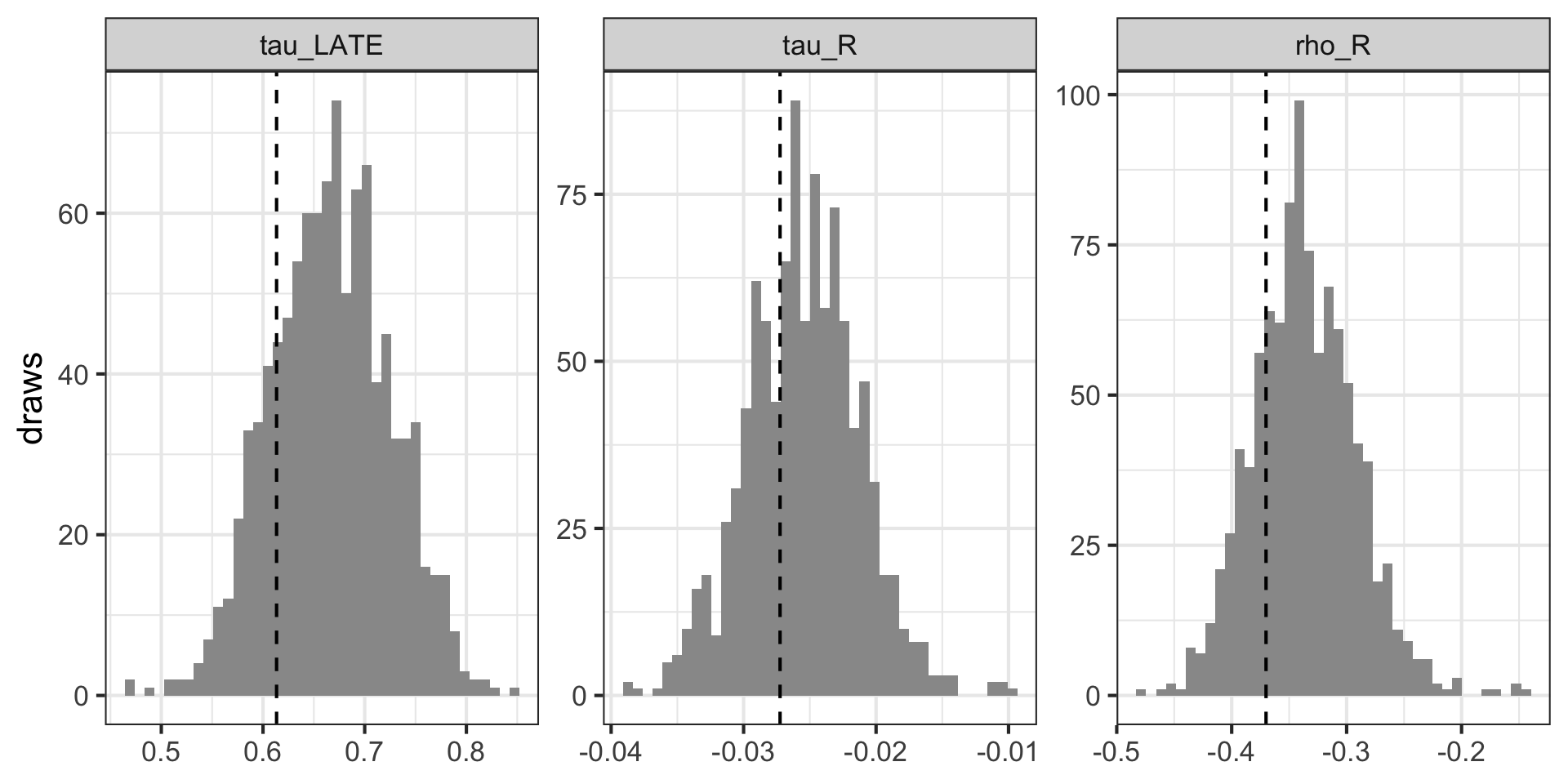
Figure 1: Posteriors of the three effects. The dashed line is the truth.

Figure 1 shows the three posteriors. The product manager’s answer is the share of draws in which rebuffers per play fall by at least 10%. We also ask for larger cuts:

c(`P(rho_R < -10%)` = mean(post[, "rho_R"] < -0.10),
  `P(rho_R < -20%)` = mean(post[, "rho_R"] < -0.20),
  `P(rho_R < -30%)` = mean(post[, "rho_R"] < -0.30),
  `P(tau_LATE > 0)` = mean(post[, "tau_LATE"] > 0))

P(rho_R < -10%) P(rho_R < -20%) P(rho_R < -30%) P(tau_LATE > 0) 
          1.000           0.995           0.798           1.000 

Every draw has rebuffers per play falling by at least 10%, so the posterior probability is 1.000 up to the resolution of 1,000 draws. A cut of at least 20% has probability 0.995, and a cut of at least 30% has probability 0.80. None of these numbers needed a delta method or a joint covariance: \(\rho_R\) was computed on each draw, like the other effects.

Does the posterior agree with the sandwich?

The posterior standard deviations in Table 1 are close to the previous post’s standard errors: 0.0583 against 0.0572 for the LATE, and 0.00424 against 0.00410 for the ratio. With 1,000 draws, a posterior standard deviation carries Monte Carlo noise of about \(1/\sqrt{2 \cdot 999} \approx 2\%\). Why should they agree?

The bootstrap post linearized a weighted least squares draw around the estimate and found the sandwich. The same argument works here. A draw is a smooth function of the weighted sums over accounts, and each weighted sum moves from its value at \(\xi = 1\) by \(\sum_a (\xi_a - 1) \times\) (the account’s contribution). To first order, an effect’s draw is

\[\tau^{(b)} - \hat\tau \approx \sum_a (\xi^{(b)}_a - 1)\, \psi_a,\]

where \(\psi_a\) is account \(a\)’s influence on the effect, the change in \(\hat\tau\) per unit change in the account’s weight. The bootstrap weights are independent with variance 1, so the posterior variance is approximately \(\sum_a \psi_a^2\), a sum of squared influences over accounts. The previous post’s cluster robust variance is also a sum of squared influences over accounts, with one difference: it held \(\hat e_{\text{day}}\) and \(\bar x_C\) fixed, so its \(\psi_a\) only describes how the account moves \(\hat\beta\). The bootstrap also moves the propensities and the compliers’ mean. Taddy et al. (2016) show the same first order equivalence for least squares in digital experiments.

How much do the extra terms matter? We rerun the same draws with the compliers’ mean held at its estimate.

draw_fixed_x_C <- function(rows, xi, x_C_c) {
  acc <- rows$accounts
  e_day <- rowsum(xi * acc$Z, acc$day)[, 1] / rowsum(xi, acc$day)[, 1]
  w_ap <- (xi * if_else(acc$Z == 1, 1 / e_day[acc$day], 1 / (1 - e_day[acc$day])))[rows$account]
  beta <- solve(crossprod(rows$M_1 * w_ap, rows$M_2), crossprod(rows$M_1 * w_ap, rows$Y))
  colnames(beta) <- y_cols
  effect_values(beta, x_C_c)
}
post_fixed <- map(seq_len(B), \(b) draw_fixed_x_C(rows, Xi[, b], x_C - x_ref)) |>
  do.call(what = rbind)
rbind(`previous post: se` = c(css$se, NA),
      `posterior sd, x_C held fixed` = apply(post_fixed, 2, sd),
      `posterior sd` = apply(post, 2, sd))

                               tau_LATE       tau_R      rho_R
previous post: se            0.05716055 0.004104151         NA
posterior sd, x_C held fixed 0.05662123 0.004216914 0.04443268
posterior sd                 0.05830711 0.004242300 0.04483163

Holding the compliers’ mean fixed brings the posterior standard deviation of the LATE to 0.0566, close to the sandwich. So the uncertainty in \(\bar x_C\), which the delta method of the previous post left out, accounts for the difference in this experiment. The appendix shows over 1,000 simulated experiments that the difference is small on average, and that both are calibrated. The bootstrap includes it without any extra derivation.

Checking every design

The previous post showed that turning off the encouragement, the clusters or the ramp gives the textbook analysis of a simpler design. The posterior should follow along: with the encouragement off, the compliers are everyone and \(\bar x_C\) is the weighted mean of \(x\); with the clusters off, each account has one profile, so the bootstrap weights are per profile; with the ramp off, the inverse propensity weights are 1. Table 2 compares, for each of the 8 combinations, the posterior mean and standard deviation of the LATE with the estimate and standard error of the textbook model from estimatr, and the ratio’s posterior standard deviation with the universal model’s sandwich. Each posterior has 500 draws, to keep this check fast, so each posterior standard deviation carries Monte Carlo noise of about 3%.

textbook <- function(df, x_C, clustered, encouraged, outcome, covs = x_cols) {
  df_c <- df |>
    mutate(across(all_of(covs), \(v) v - x_C[cur_column()]))     # coefficient on T is the line at x_C
  rhs <- paste0("(", paste(covs, collapse = " + "), ")")
  f <- as.formula(if (encouraged) paste(outcome, "~", rhs, "* T |", rhs, "* Z") else paste(outcome, "~", rhs, "* T"))
  estimator <- if (encouraged) iv_robust else lm_robust
  fit <- if (clustered) estimator(f, data = df_c, weights = w, clusters = account, se_type = "CR0")
         else estimator(f, data = df_c, weights = w, se_type = "HC0")
  c(estimate = fit$coefficients[["T"]], se = fit$std.error[["T"]])
}

check_design <- function(encouraged, clustered, ramp) {
  set.seed(7)
  df <- simulate_accounts(propensity = if (ramp) propensity else rep(0.3, 4), full_compliance = !encouraged,
                          one_profile = !clustered) |>
    prepare(ramp = ramp)
  x_C <- complier_mean(df)
  tb <- textbook(df, x_C, clustered, encouraged, "y")
  css <- effects(fit_rows(df), x_C, x_ref)
  rows <- rows_data(df)
  post <- map(1:500, \(b) draw_rows(rows, rexp(nrow(rows$accounts)), ramp, encouraged)) |>
    do.call(what = rbind)
  tibble(encouraged, clustered, ramp,
         textbook = tb[["estimate"]], posterior_mean = mean(post[, "tau_LATE"]),
         textbook_se = tb[["se"]], posterior_sd = sd(post[, "tau_LATE"]),
         ratio_se = css$se[2], ratio_posterior_sd = sd(post[, "tau_R"]))
}

design_tab <- expand_grid(encouraged = c(FALSE, TRUE), clustered = c(FALSE, TRUE), ramp = c(FALSE, TRUE)) |>
  pmap_dfr(check_design)

design_tab |>
  mutate(across(c(encouraged, clustered, ramp), \(v) if_else(v, "yes", "no"))) |>
  kable(digits = 4, col.names = c("Encouragement", "Clusters", "Ramp", "LATE: textbook", "LATE: posterior mean",
                                  "LATE: textbook SE", "LATE: posterior SD", "Ratio: sandwich SE", "Ratio: posterior SD"))

Table 2: Eight designs. For the LATE, the textbook estimate and standard error from estimatr against the posterior mean and standard deviation. For the ratio, the universal model’s sandwich standard error against the posterior standard deviation.

Encouragement	Clusters	Ramp	LATE: textbook	LATE: posterior mean	LATE: textbook SE	LATE: posterior SD	Ratio: sandwich SE	Ratio: posterior SD
no	no	no	0.5574	0.5577	0.0208	0.0209	0.0016	0.0017
no	no	yes	0.5817	0.5803	0.0359	0.0362	0.0026	0.0027
no	yes	no	0.5415	0.5411	0.0154	0.0159	0.0011	0.0011
no	yes	yes	0.5347	0.5361	0.0263	0.0252	0.0017	0.0017
yes	no	no	0.5916	0.5903	0.0441	0.0459	0.0033	0.0034
yes	no	yes	0.6339	0.6299	0.0777	0.0780	0.0059	0.0056
yes	yes	no	0.6242	0.6249	0.0349	0.0356	0.0025	0.0026
yes	yes	yes	0.6108	0.6091	0.0576	0.0566	0.0041	0.0041

In every design the posterior is centered at the textbook estimate, up to the Monte Carlo noise of 500 draws, and its standard deviation is close to the textbook standard error. The first row is a purely randomized AB test with one row per user and a mean metric, where the Bayesian bootstrap of Lin’s regression gives the heteroskedasticity robust standard error, as in the bootstrap post. The last row is our experiment.

The weight must go on the account

What if we ignore the clusters, and draw a bootstrap weight for each profile instead of each account? draw_rows can do that if we pretend that every profile is its own account.

rows_profile <- df |>
  mutate(account = row_number()) |>
  rows_data()
set.seed(3)
post_profile <- map(seq_len(B), \(b) draw_rows(rows_profile, rexp(nrow(df)))) |>
  do.call(what = rbind)
rbind(`weights per account` = apply(post, 2, sd), `weights per profile` = apply(post_profile, 2, sd))

                      tau_LATE       tau_R      rho_R
weights per account 0.05830711 0.004242300 0.04483163
weights per profile 0.05348719 0.003958555 0.04141338

Weights per profile make the posterior of the LATE 8% narrower. Profiles of the same account share network quality and engagement, so they are not independent, and a population that mixes profiles freely is more certain than the data justify. This is the posterior counterpart of using a heteroskedasticity robust standard error where a cluster robust one is needed. The appendix confirms over 1,000 simulated experiments that weights per profile under-cover the LATE, while weights per account are calibrated.

The Bayesian bootstrap of the universal model is the universal model fit with one more weight per account. It gives a posterior for every effect of every design that the model covers, and for any function of those effects.

Efficient Computation

The posterior took 12.7 seconds: 1,000 fits on 43,989 profile rows. Each draw reads every profile row, so an experiment with hundreds of millions of profile rows would need 1,000 passes over the data. The previous post reduced a single fit to one pass and a compressed dataset of 8 rows. Can we do the same for the posterior?

The compressed rows cannot be reweighted

The tempting shortcut is to apply the Bayesian bootstrap to the compressed dataset: draw one bootstrap weight per compressed row and refit. That would treat the 8 strata as the units of independence. A population would then be a mix of 8 kinds of strata, and the posterior would describe uncertainty about the strata’s shares, not about the accounts within them. Within a stratum, every account would always count the same, so the posterior would not see how much the accounts vary. By (A1) the unit is the account, and a compressed row has already added the accounts together.

What one draw needs

Look again at what a draw computes. Each step of draw_rows adds up profile rows with the combined weight \(\xi_a w_a\), and \(w_a\) is the same for all accounts of a stratum. Grouping the profiles by account and the accounts by stratum, the sums of a draw are sums over strata of the stratum’s inverse propensity weight times

\[\sum_{a \in h} \xi_a \begin{pmatrix} 1 \\ u_a \end{pmatrix}.\]

The first entry, \(\sum_{a \in h} \xi_a\), is the stratum’s total bootstrap weight, which gives the propensities. The rest is the bootstrap-weighted sum of the account summaries, which gives \(\beta\) and \(\bar x_C\), exactly as \(\sum_{a \in h} u_a\) gave them in the previous post. We write \(v_a = (1, u_a)\) for the account summary with a 1 in front. One draw needs one weighted sum \(\sum_{a \in h} \xi_a v_a\) per stratum. fit_sums computes the three effects from these 8 sums.

fit_sums <- function(keys, sums, ramp = TRUE, encouraged = TRUE) {
  # keys: Z and day of each stratum; sums: one row per stratum, sum of xi_a v_a
  total <- sums[, 1]                                            # total bootstrap weight of the stratum
  e_day <- (tapply(total * keys$Z, keys$day, sum) / tapply(total, keys$day, sum))[as.character(keys$day)]
  w <- if (ramp) ifelse(keys$Z == 1, 1 / e_day, 1 / (1 - e_day)) else rep(1, nrow(keys))
  s <- colSums(sums[, -1] * w)                                  # all strata
  s_Z <- colSums(sums[, -1] * (w * keys$Z))                     # prompted strata
  i_Y <- 1:(d * o)
  i_S <- d * o + 1:(d * d)
  i_T <- d * o + d * d + 1:(d * d)
  block <- \(v, i, ncol = d) matrix(v[i], ncol = ncol)
  M1_W_M2 <- rbind(cbind(block(s, i_S), block(s, i_T)), cbind(block(s_Z, i_S), block(s_Z, i_T)))
  M1_W_Y <- rbind(block(s, i_Y, o), block(s_Z, i_Y, o))
  beta <- solve(M1_W_M2, M1_W_Y)
  colnames(beta) <- y_cols
  x_C_c <- if (encouraged) {
    s_0 <- s - s_Z                                              # unprompted strata
    diff <- block(s_Z, i_T)[, 1] / s_Z[i_S][1] - block(s_0, i_T)[, 1] / s_0[i_S][1]
    diff[-1] / diff[1]
  } else block(s, i_S)[-1, 1] / s[i_S][1]
  effect_values(beta, x_C_c)
}

The sums \(\sum_{a \in h} \xi_a v_a\) change with every draw, and the compressed dataset of the previous post kept only \(\sum_{a \in h} v_a\) and \(\sum_{a \in h} v_a v_a^\top\), which are the same for every draw. There are two ways forward. We can compute the weighted sums of all \(B\) draws in one pass over the profile rows. Or we can ask what the compressed dataset already tells us about them.

Exact: draw the weights during the compression pass

The previous post built each account summary \(u_a\) in one pass over the profile rows, added it into its stratum’s sums, and discarded it. We change one line: instead of adding \(u_a\) once, we add \(\xi^{(b)}_a v_a\) for every draw \(b\). The pass then produces, for every stratum, a \(B \times (1 + \dim u_a)\) matrix whose row \(b\) is the weighted sum of draw \(b\).

The weights must be the same wherever the account is processed, and drawing them must not require knowing the other accounts. We compute \(\xi^{(b)}_a\) from a hash of the account id and the draw number, turned into a uniform number \(U\) and then into an Exponential(1) weight, \(-\log U\). Any machine that holds account \(a\) draws the same weights, as with the Poisson bootstrap. The kernel is written in C++ with Rcpp, like the compression kernel of the previous post. It also contains compress_moments, which builds the compressed dataset of the previous post in the same layout, which we use in the next section.

#include <Rcpp.h>
#include <vector>
#include <cmath>
#include <cstdint>
using namespace Rcpp;

// The bootstrap weight of account a in draw b: a hash of (seed, a, b) turned into an Exponential(1) number.
// Every machine that holds account a computes the same weight, without knowing the other accounts.
inline double xi_weight(uint64_t seed, uint64_t a, uint64_t b) {
  uint64_t z = seed + 0x9E3779B97F4A7C15ULL * (a * 1000003ULL + b + 1);
  z = (z ^ (z >> 30)) * 0xBF58476D1CE4E5B9ULL;
  z = (z ^ (z >> 27)) * 0x94D049BB133111EBULL;
  z = z ^ (z >> 31);
  double U = ((z >> 11) + 0.5) / 9007199254740992.0;          // uniform on (0, 1)
  return -std::log(U);
}

// [[Rcpp::export]]
NumericMatrix bootstrap_weights(IntegerVector account, int B, double seed) {
  NumericMatrix xi(account.size(), B);
  for (int a = 0; a < account.size(); a++)
    for (int b = 0; b < B; b++) xi(a, b) = xi_weight((uint64_t) seed, account[a], b);
  return xi;
}

// Add profile row i into the account summary u = (vec S^Y, vec S, vec S^T), with R = (1, x) and Y the outcome columns.
inline void add_row(std::vector<double>& u, const NumericMatrix& R, const NumericVector& T, const NumericMatrix& Y, int i) {
  int d = R.ncol(), o = Y.ncol();
  for (int l = 0; l < o; l++) for (int j = 0; j < d; j++) u[l * d + j] += R(i, j) * Y(i, l);
  for (int m = 0; m < d; m++) for (int j = 0; j < d; j++) {
    double rr = R(i, j) * R(i, m);
    u[d * o + m * d + j] += rr;
    u[d * o + d * d + m * d + j] += T[i] * rr;
  }
}

// One pass over the profile rows, which must be grouped by account. For every stratum, row b of the output
// is the weighted sum of v_a = (1, u_a) over its accounts, with the bootstrap weights of draw b.
// [[Rcpp::export]]
List compress_bootstrap(IntegerVector account, IntegerVector stratum, NumericMatrix R, NumericVector T,
                        NumericMatrix Y, int n_strata, int B, double seed) {
  int n = R.nrow(), d = R.ncol(), o = Y.ncol(), q = d * o + 2 * d * d;
  std::vector<double> u(q, 0.0), xi(B);
  std::vector<int> nz;
  std::vector<NumericMatrix> sums;
  for (int h = 0; h < n_strata; h++) sums.push_back(NumericMatrix(B, q + 1));
  auto add_account = [&](int a, int h) {
    for (int b = 0; b < B; b++) xi[b] = xi_weight((uint64_t) seed, a, b);   // the account's B weights
    nz.clear();
    for (int k = 0; k < q; k++) if (u[k] != 0) nz.push_back(k);
    double* S = sums[h].begin();                                            // column k + 1 holds entry k of u
    for (int b = 0; b < B; b++) S[b] += xi[b];
    for (int k : nz) {
      double* col = S + (size_t) (k + 1) * B;
      for (int b = 0; b < B; b++) col[b] += xi[b] * u[k];
    }
    for (int k : nz) u[k] = 0;
  };
  for (int i = 0; i < n; i++) {
    if (i > 0 && account[i] != account[i - 1]) add_account(account[i - 1], stratum[i - 1] - 1);
    add_row(u, R, T, Y, i);
  }
  add_account(account[n - 1], stratum[n - 1] - 1);
  List out(n_strata);
  for (int h = 0; h < n_strata; h++) out[h] = sums[h];
  return out;
}

// One pass over the profile rows to the compressed dataset: per stratum, sum v_a and sum v_a v_a^T.
// [[Rcpp::export]]
List compress_moments(IntegerVector account, IntegerVector stratum, NumericMatrix R, NumericVector T,
                      NumericMatrix Y, int n_strata) {
  int n = R.nrow(), d = R.ncol(), o = Y.ncol(), q = d * o + 2 * d * d;
  std::vector<double> v(q + 1, 0.0);
  std::vector<int> nz;
  std::vector<NumericVector> first;
  std::vector<NumericMatrix> second;
  for (int h = 0; h < n_strata; h++) { first.push_back(NumericVector(q + 1)); second.push_back(NumericMatrix(q + 1, q + 1)); }
  auto add_account = [&](int h) {
    v[0] = 1;
    nz.clear();
    for (int k = 0; k <= q; k++) if (v[k] != 0) nz.push_back(k);
    NumericMatrix& S2 = second[h];
    for (size_t i = 0; i < nz.size(); i++) {
      first[h][nz[i]] += v[nz[i]];
      for (size_t j = i; j < nz.size(); j++) S2(nz[j], nz[i]) += v[nz[i]] * v[nz[j]];   // lower triangle
    }
    for (int k : nz) v[k] = 0;
  };
  std::vector<double> u(q, 0.0);
  for (int i = 0; i < n; i++) {
    if (i > 0 && account[i] != account[i - 1]) {
      for (int k = 0; k < q; k++) { v[k + 1] = u[k]; u[k] = 0; }
      add_account(stratum[i - 1] - 1);
    }
    add_row(u, R, T, Y, i);
  }
  for (int k = 0; k < q; k++) v[k + 1] = u[k];
  add_account(stratum[n - 1] - 1);
  List out(n_strata);
  for (int h = 0; h < n_strata; h++) {
    NumericMatrix& S2 = second[h];
    for (int i = 0; i <= q; i++) for (int j = i + 1; j <= q; j++) S2(i, j) = S2(j, i);
    out[h] = List::create(_["first"] = first[h], _["second"] = S2);
  }
  return out;
}

strata numbers the strata, and posterior_one_pass runs the kernel and turns each draw’s 8 weighted sums into effects.

strata <- function(df) {
  accounts <- df |>
    distinct(account, Z, day) |>
    arrange(account)
  keys <- accounts |>
    distinct(Z, day) |>
    arrange(Z, day)
  list(keys = keys, h = match(paste(accounts$Z, accounts$day), paste(keys$Z, keys$day)))
}

posterior_one_pass <- function(df, B, seed) {
  st <- strata(df)
  sums <- compress_bootstrap(df$account, st$h[df$account], centered(df), df$T, as.matrix(df[y_cols]),
                             nrow(st$keys), B, seed)
  posterior_from_sums(st$keys, sums)
}

posterior_from_sums <- function(keys, sums) {      # sums: one B x (1 + q) matrix per stratum
  all_strata <- do.call(cbind, sums)                # row b holds draw b of every stratum, side by side
  map(seq_len(nrow(all_strata)), \(b) fit_sums(keys, matrix(all_strata[b, ], nrow = length(sums), byrow = TRUE))) |>
    do.call(what = rbind)
}

st <- strata(df)
sums <- compress_bootstrap(df$account, st$h[df$account], centered(df), df$T, as.matrix(df[y_cols]),
                           nrow(st$keys), B, 2026)
length(sums)

[1] 8

dim(sums[[1]])

[1] 1000  103

round(sums[[1]][1:3, 1:5], 2)

        [,1]     [,2]     [,3]    [,4]    [,5]
[1,] 7640.81 39343.22 38801.70 9059.22 5441.00
[2,] 7643.83 38856.08 39765.03 6802.07 5277.70
[3,] 7665.45 38934.50 42210.67 6959.21 5104.34

There is one matrix per stratum, with one row per draw and 1 + 102 columns: the total bootstrap weight, followed by the weighted sums of the entries of \(u_a\). The first column of the first stratum, the unprompted accounts of day 1, is its total bootstrap weight in each draw. It hovers around the stratum’s 7639 accounts, with a standard deviation of about \(\sqrt{7639}\), because the weights are independent with mean and variance 1. The next columns start the hours block of \(S^Y\): the weighted sums of the hours and of the hours times each centered covariate.

To check the kernel, we feed the same bootstrap weights to draw_rows on the profile rows and compare the first 20 draws.

post_one_pass <- posterior_one_pass(df, B, 2026)
Xi_hash <- bootstrap_weights(rows$accounts$account, 20, 2026)
post_rows_hash <- map(1:20, \(b) draw_rows(rows, Xi_hash[, b])) |>
  do.call(what = rbind)
max(abs(post_one_pass[1:20, ] - post_rows_hash))

[1] 3.309575e-13

The two agree to floating point rounding. One pass over the profile rows gives the exact Bayesian bootstrap. The cost is that every account is multiplied into \(B\) sums instead of one, and the output has \(B\) rows per stratum instead of one.

From the compressed dataset: the compressed row is the posterior’s moments

Do we need a new pass at all? The compressed dataset of the previous post holds, for each stratum, \(\sum_{a \in h} v_a\) and \(\sum_{a \in h} v_a v_a^\top\). Given the data, the account summaries are fixed and only the bootstrap weights are random. The weights are independent, with mean 1 and variance 1, so

\[\begin{align} E\Big[\sum_{a \in h} \xi_a v_a \,\Big|\, \text{data}\Big] &= \sum_{a \in h} E[\xi_a]\, v_a = \sum_{a \in h} v_a, \\ \text{Cov}\Big(\sum_{a \in h} \xi_a v_a \,\Big|\, \text{data}\Big) &= \sum_{a \in h} \text{Var}(\xi_a)\, v_a v_a^\top = \sum_{a \in h} v_a v_a^\top, \end{align}\]

where the covariance has no cross terms between accounts because their weights are independent. The mean and the covariance of the weighted sums that a draw needs are exactly the two fields of the compressed row. The count \(G_h\) is there too, as the first entry of \(\sum_{a \in h} v_a\), since the first entry of \(v_a\) is 1. The second moments are not centered, because the randomness comes from the weights varying around 1, not from the accounts varying around their mean. Weights of different strata are independent, so the weighted sums of different strata are independent.

The compressed row has the first two moments of the weighted sums, but not their whole distribution. Each weighted sum adds up hundreds or thousands of independent terms \(\xi_a v_a\), one per account: the smallest stratum, the prompted accounts of day 1, has 412 accounts. By the central limit theorem, each sum is approximately normal. So we draw the sum of each stratum from the normal distribution with the compressed row’s mean and covariance, and push every draw through fit_sums. Only the weighted sums are approximated as normal. The fit, the propensities, the compliers’ mean and the ratios are computed exactly from each draw, so the posterior can still be skewed when the effects are nonlinear functions of the sums.

posterior_compressed <- function(moments, keys, B) {
  # One normal draw of the weighted sums per stratum and draw: mean sum v_a, covariance sum v_a v_a^T
  draws <- map(moments, \(m) {
    root <- eigen(m$second, symmetric = TRUE)
    A <- root$vectors %*% diag(sqrt(pmax(root$values, 0)))
    sweep(matrix(rnorm(B * ncol(A)), B) %*% t(A), 2, m$first, `+`)          # B x (1 + q)
  })
  posterior_from_sums(keys, draws)
}

moments <- compress_moments(df$account, st$h[df$account], centered(df), df$T, as.matrix(df[y_cols]), nrow(st$keys))
map_dbl(moments, \(m) m$first[1])                                            # G_h, the accounts per stratum

[1] 7639 5321 2988 1014  412  634  981 1011

set.seed(4)
post_compressed <- posterior_compressed(moments, st$keys, B)

The eigen call computes a square root of each stratum’s covariance. A Cholesky factorization would also work, except that \(u_a\) repeats the off-diagonal entries of the symmetric blocks \(S_a\) and \(S^T_a\), which makes the covariance singular.

The two posteriors come from different random numbers, so we compare them with \(10{,}000\) draws each, to keep the Monte Carlo noise of each standard deviation below 1%.

B_compare <- 10000
time_one_pass <- system.time(post_exact_10k <- posterior_one_pass(df, B_compare, 2027))[["elapsed"]]
set.seed(5)
time_compressed <- system.time(post_compressed_10k <- posterior_compressed(moments, st$keys, B_compare))[["elapsed"]]
skew <- \(v) mean((v - mean(v))^3) / sd(v)^3
summary_tab <- \(p, method) tibble(method = method, effect = colnames(p), mean = colMeans(p), sd = apply(p, 2, sd),
                                 `2.5%` = apply(p, 2, quantile, 0.025), `97.5%` = apply(p, 2, quantile, 0.975),
                                 skewness = apply(p, 2, skew))
compare_tab <- bind_rows(summary_tab(post_exact_10k, "exact, one pass"),
                         summary_tab(post_compressed_10k, "from the compressed dataset")) |>
  arrange(factor(effect, levels = colnames(post)), method)

compare_tab |>
  kable(digits = 4)

Table 3: The exact posterior from one pass over the profile rows, and the posterior from the compressed dataset, with 10,000 draws each.

method	effect	mean	sd	2.5%	97.5%	skewness
exact, one pass	tau_LATE	0.6631	0.0581	0.5490	0.7758	-0.0162
from the compressed dataset	tau_LATE	0.6636	0.0587	0.5499	0.7786	-0.0001
exact, one pass	tau_R	-0.0255	0.0041	-0.0335	-0.0172	0.0945
from the compressed dataset	tau_R	-0.0254	0.0042	-0.0338	-0.0173	-0.0062
exact, one pass	rho_R	-0.3368	0.0439	-0.4179	-0.2446	0.2908
from the compressed dataset	rho_R	-0.3360	0.0442	-0.4194	-0.2466	0.1832

probs <- seq(0.005, 0.995, by = 0.005)
map_dfr(colnames(post), \(eff) tibble(effect = eff,
                                      exact = quantile(post_exact_10k[, eff], probs),
                                      compressed = quantile(post_compressed_10k[, eff], probs))) |>
  mutate(effect = factor(effect, levels = colnames(post))) |>
  ggplot(aes(x = exact, y = compressed)) +
  geom_abline(color = "grey50") +
  geom_point(size = 1, color = "#0072B2") +
  facet_wrap(~effect, scales = "free") +
  scale_x_continuous(n.breaks = 3) +
  labs(x = "exact posterior quantile", y = "compressed posterior quantile") +
  theme_bw(base_size = 16)

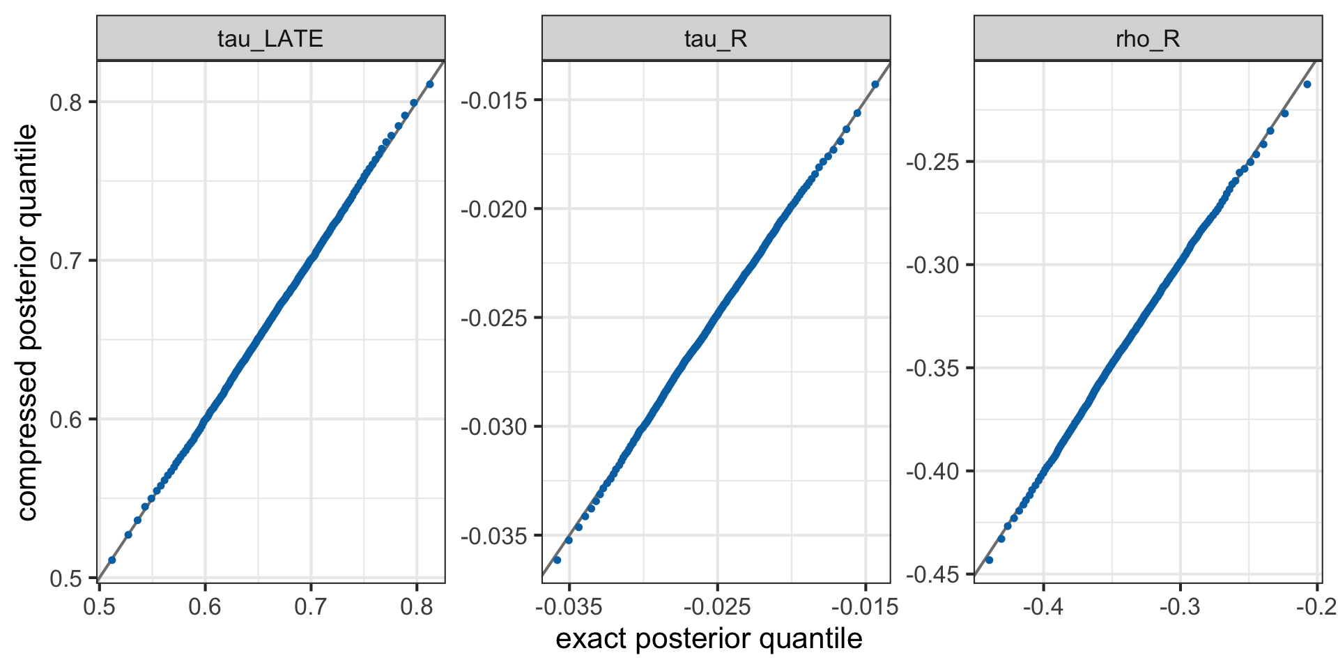
Figure 2: Quantiles of the posterior from the compressed dataset against quantiles of the exact posterior, 10,000 draws each. Points on the line mean the two posteriors agree.

Table 3 and Figure 2 show that the two posteriors agree. For the LATE, the posterior standard deviations are 0.0581 and 0.0587, and the quantiles fall on the line, including the tails. What the normal approximation drops is the third moment of the weighted sums. The Exponential(1) weights are skewed, with a third central moment of 2, so the exact sums lean slightly to the right, and the compressed dataset does not keep the third moments \(\sum_{a \in h} v_a^{\otimes 3}\) that would describe it. In our experiment this is visible only in the skewness column. The exact posterior of \(\rho_R\) has a skewness of 0.29 and the compressed one 0.18: most of the skew comes from \(\rho_R\) being a ratio, which the exact fit of every draw keeps, and the rest from the weights, which the normal approximation drops. With very heavy-tailed accounts, such as a few whales that dominate a stratum, the weighted sums are less normal, and Taddy et al. (2016) found skewed posteriors in an experiment with 13 million users. There the exact pass is the safer choice.

There is another way to read the compressed posterior. Drawing the weighted sums from a normal with mean \(\sum_a v_a\) and covariance \(\sum_a v_a v_a^\top\) gives exactly the same distribution as weighting each account by an independent N(1, 1) number instead of an Exponential(1) number, because a weighted sum of fixed vectors with normal weights is normal. That is a multiplier bootstrap with normal weights. Its weights have the same mean and variance as the Bayesian bootstrap’s, which is why the two agree, but a normal weight can be negative, so a draw is no longer a population. We use the Gaussian draws as an approximation of the Bayesian bootstrap posterior, not as a posterior of their own.

Compute and storage

To compare the costs, we run the same simulation with a million accounts, and time the three ways to get 1,000 draws: refitting on the profile rows, the exact one pass, and the compressed dataset. Refitting on the profile rows takes too long to run in full, so we time 20 draws and multiply by 50.

set.seed(1)
big <- simulate_accounts(1e6) |>
  prepare()
st_big <- strata(big)
t_rows <- 50 * system.time({
  rows_big <- rows_data(big)
  walk(1:20, \(b) draw_rows(rows_big, rexp(nrow(rows_big$accounts))))
})[["elapsed"]]
rm(rows_big)
t_one_pass <- system.time(posterior_one_pass(big, 1000, 1))[["elapsed"]]
t_compressed <- system.time({
  moments_big <- compress_moments(big$account, st_big$h[big$account], centered(big), big$T,
                                  as.matrix(big[y_cols]), nrow(st_big$keys))
  posterior_compressed(moments_big, st_big$keys, 1000)
})[["elapsed"]]
n_big <- nrow(big)
rm(big, moments_big, st_big)
invisible(gc())

tibble(method = c("refit on the profile rows, 1,000 passes", "exact, one pass", "from the compressed dataset"),
       seconds = c(t_rows, t_one_pass, t_compressed)) |>
  kable(digits = 1, col.names = c("Method", "Seconds"))

Table 4: Seconds for 1,000 posterior draws of the three effects, on a million accounts, starting from the profile rows. The first row is extrapolated from 20 draws.

Method	Seconds
refit on the profile rows, 1,000 passes	677.8
exact, one pass	11.7
from the compressed dataset	1.2

Table 4 shows the times on the machine that rendered this post, for 2,189,477 profile rows. Refitting on the profile rows reads all of them for every draw. The exact one pass reads them once, but multiplies every account into 1,000 sums. The compressed dataset reads them once and multiplies every account into its outer product, which here is cheaper, and its 1,000 draws then never touch the profile rows.

The two efficient methods also keep different amounts of data. Write \(q = (k+1) o + (k+1)(k+2)\) for the number of distinct entries of \(u_a\), as in the previous post, where symmetric blocks count once. The exact one pass keeps \(B (1 + q)\) numbers per stratum. The compressed dataset keeps the distinct entries of \(\sum_{a \in h} v_a v_a^\top\), which is \((q+1)(q+2)/2\) numbers per stratum, and it already contains \(G_h\) and \(\sum_{a \in h} v_a\) as its first row. The first grows like \(B k^2\), the second like \(k^4\).

n_strata <- nrow(st$keys)
q_distinct <- \(k) (k + 1) * o + (k + 1) * (k + 2)
storage_tab <- tibble(k = c(3, 5, 10, 25, 50)) |>
  mutate(rows = nrow(df) * (4 + k + 3),                                   # account, Z, day, T, covariates, raw outcomes
         one_pass = n_strata * 1000 * (1 + q_distinct(k)),
         compressed = n_strata * (q_distinct(k) + 1) * (q_distinct(k) + 2) / 2)
storage_tab |>
  mutate(across(-k, \(v) format(v, big.mark = ","))) |>
  kable(col.names = c("Covariates $k$", "Numbers in the profile rows", "Exact, one pass", "Compressed dataset"))

Table 5: Numbers kept by each method with 8 strata, 5 outcome columns and 1,000 draws, counting each distinct number once, against the numbers in the profile rows of our experiment.

Covariates \(k\)	Numbers in the profile rows	Exact, one pass	Compressed dataset
3	439,890	328,000	6,888
5	527,868	584,000	21,608
10	747,813	1,504,000	142,128
25	1,407,648	6,664,000	2,778,888
50	2,507,373	23,264,000	33,837,488

Table 5 shows the trade-off. With our 5 covariates, the compressed dataset keeps 21,608 numbers, while the exact one pass keeps 584,000, about as many as the 527,868 numbers in the profile rows of this experiment of 20,000 accounts. Neither grows with the number of accounts, so for an experiment with a million accounts both are much smaller than the data. The two cross near \(q = 2B\): with 50 covariates the compressed dataset keeps more than the exact one pass. With prognostic scores, the previous post’s recommendation for many covariates, \(k\) stays at one score per raw outcome, and the compressed dataset stays small.

The choice between the two:

1. The compressed dataset is the default. It is the same compressed dataset that the previous post stores for standard errors, so a platform that already keeps it gets the posterior for free, for any number of draws and any function of the effects, without reading the profile rows again. Its only approximation is the normality of each stratum’s weighted sum.
2. The exact one pass is for strata with few accounts or very heavy-tailed accounts, where the weighted sums are not normal, or when an exact posterior is required. It needs the number of draws, and the seed, before the pass.

Summary

The universal model of the previous post gets a posterior with one more weight. Under the assumptions of the design and of the Bayesian bootstrap, a draw of the population gives each account an Exponential(1) bootstrap weight, shared by its profiles, and the universal model is refit with the combined weight. The propensities and the compliers’ mean are recomputed in every draw, and every effect, including ratios and relative changes, is computed on the draw. The result is a posterior for the LATE, the ratio and any function of them, in every design the universal model covers, and the posterior agrees with the sandwich standard errors and with textbook fits of the simpler designs. The weight must go on the account: weights on profiles give a posterior that is too narrow.

The posterior does not need the profile rows once per draw. Each draw needs only one bootstrap-weighted sum of account summaries per stratum. One pass over the profile rows, with weights drawn from a hash of the account id, computes these sums for every draw exactly. And the compressed dataset of the previous post already holds the mean and covariance of these sums, so a posterior can be drawn from it directly, with a normal approximation for each stratum’s sum and the exact nonlinear fit for every draw.

Appendix

Monte Carlo

We repeat the experiment 1,000 times. In each one we compute the previous post’s estimates and standard errors, and three posteriors with 500 draws each: the exact posterior with weights per account, from the one pass; the posterior with weights per profile, from the same pass with every profile treated as its own account; and the posterior from the compressed dataset. A 95% credible interval is the 2.5% and 97.5% quantiles of the draws. A posterior is not required to cover the truth in 95% of experiments, but when the posterior’s spread matches the sampling variability of the estimate, as the linearization argument says it should, it does. The SE/SD column divides the average standard error, or the average posterior standard deviation, by the standard deviation of the estimates across experiments.

analyze <- function(seed, B = 500) {
  set.seed(seed)
  df <- simulate_accounts() |>
    prepare()
  css <- effects(fit_rows(df), complier_mean(df), x_ref)
  st <- strata(df)
  moments <- compress_moments(df$account, st$h[df$account], centered(df), df$T, as.matrix(df[y_cols]), nrow(st$keys))
  posteriors <- list(
    "weights per account, exact" = posterior_one_pass(df, B, seed),
    "weights per profile" = posterior_one_pass(mutate(df, account = row_number()), B, seed),
    "weights per account, compressed dataset" = posterior_compressed(moments, st$keys, B))
  bind_rows(
    tibble(effect = css$effect, method = "previous post: estimate and SE", estimate = css$estimate, spread = css$se,
           lo = css$estimate - qnorm(0.975) * css$se, hi = css$estimate + qnorm(0.975) * css$se),
    imap_dfr(posteriors, \(p, name) tibble(effect = colnames(p), method = name, estimate = colMeans(p),
                                           spread = apply(p, 2, sd), lo = apply(p, 2, quantile, 0.025),
                                           hi = apply(p, 2, quantile, 0.975)))) |>
    mutate(rep = seed)
}
rm(Xi, post_fixed, post_profile, rows_profile)
invisible(gc())
mc <- mclapply(1:1000, analyze, mc.cores = cores) |>
  bind_rows()
mc_tab <- mc |>
  mutate(target = truth[effect]) |>
  group_by(effect, method) |>
  summarise(bias = mean(estimate - target), sd = sd(estimate), se_over_sd = mean(spread) / sd(estimate),
            coverage = mean(lo <= target & target <= hi), .groups = "drop") |>
  arrange(factor(effect, levels = names(truth)), method)

mc_tab |>
  kable(digits = 4, col.names = c("Effect", "Method", "Bias", "SD", "SE/SD", "Coverage"))

Table 6: 1,000 simulated experiments. Bias and SD are of the estimate or the posterior mean. SE/SD compares the average standard error or posterior standard deviation with the SD, and coverage is the share of 95% intervals that contain the truth.

Effect	Method	Bias	SD	SE/SD	Coverage
tau_LATE	previous post: estimate and SE	-0.0002	0.0621	0.9629	0.945
tau_LATE	weights per account, compressed dataset	-0.0005	0.0620	0.9748	0.937
tau_LATE	weights per account, exact	-0.0002	0.0622	0.9679	0.940
tau_LATE	weights per profile	-0.0003	0.0622	0.8559	0.909
tau_R	previous post: estimate and SE	-0.0001	0.0039	1.0241	0.944
tau_R	weights per account, compressed dataset	-0.0001	0.0039	1.0268	0.948
tau_R	weights per account, exact	-0.0001	0.0039	1.0213	0.944
tau_R	weights per profile	-0.0001	0.0039	1.0115	0.946
rho_R	weights per account, compressed dataset	0.0021	0.0410	1.0277	0.944
rho_R	weights per account, exact	0.0020	0.0410	1.0227	0.942
rho_R	weights per profile	0.0021	0.0409	1.0135	0.942

With 1,000 experiments, SE/SD is uncertain by about \(1/\sqrt{2 \cdot 999} \approx 2\%\), and the coverage by about \(\sqrt{0.95 \cdot 0.05 / 1000} \approx 0.7\) percentage points. Reading Table 6:

1. With weights per account, the exact posterior and the posterior from the compressed dataset cover the LATE 94.0% and 93.7% of the time, within about one percentage point of the previous post’s standard errors, 94.5%, and of 95%. Their intervals are quantiles of only 500 draws, which adds a little noise to each interval’s endpoints. For the ratios, coverage is between 94.2% and 94.8%. The relative effect \(\rho_R\) has no row for the previous post, which did not compute it.
2. Weights per profile cover the LATE only 90.9% of the time, and their posterior standard deviation is 14% smaller than the spread of the estimates.
3. The LATE and \(\tau_R\) are unbiased, up to the Monte Carlo error of the bias, about 0.0020 for the LATE. The posterior mean of \(\rho_R\) is off by 0.0020, 1.6 Monte Carlo standard errors and 5% of a standard deviation. A ratio of estimates has a bias that shrinks like \(1/n\), faster than its standard deviation, so it does not affect the coverage.